Module 03: GEO Dataset Download & Preprocessing

1 Overview
This module performs two core tasks:
Download all HFrEF-related GEO datasets (RNA-seq, microarray, single-cell)
Preprocess only GSE141910:
- Raw counts → filtering → SVA batch correction → for DEG & WGCNA
- FPKM/TPM → SVA correction → for machine learning & hub gene validation
All other external datasets are downloaded but not preprocessed in this module.
Datasets downloaded: - RNA-seq: GSE141910, GSE116250, GSE161472, GSE135055 - Microarray: GSE120895, GSE19303 - Single-cell: GSE183852
2 Load Packages
3 Part 1: Download ALL GEO Datasets
3.1 RNA‑seq Datasets
3.1.1 GSE141910: Main training set
Code
rm(list=ls())

raw_dir <- "../../data/raw/geo/GSE141910"
if (!dir.exists(raw_dir)) dir.create(raw_dir, recursive = TRUE)

Sys.setlocale("LC_ALL", "C")
gse141910 <- getGEO("GSE141910", destdir = raw_dir, getGPL = TRUE, AnnotGPL = F)
Sys.setlocale("LC_ALL", "")

gse141910_pheno_raw <- pData(gse141910[[1]])

# url <- "https://www.dropbox.com/scl/fi/2leazyjscrvn3ahderxt9/phenoData.csv?rlkey=vo0gpy1q503ywz18mro0d5nai&e=1&dl=1"
# gse141910_pheno_raw_with_lvef <- read_csv(url)
gse141910_pheno_raw_with_lvef <- read.csv("../../data/raw/geo/GSE141910/gse141910_pheno_raw_with_lvef.csv")

url <- "https://www.ncbi.nlm.nih.gov/geo/download/?type=rnaseq_counts&acc=GSE141910&format=file&file=GSE141910_raw_counts_GRCh38.p13_NCBI.tsv.gz"
gse141910_counts_raw <- read_tsv(url)

url <- "https://www.ncbi.nlm.nih.gov/geo/download/?type=rnaseq_counts&acc=GSE141910&format=file&file=GSE141910_norm_counts_FPKM_GRCh38.p13_NCBI.tsv.gz"
gse141910_fpkm_raw <- read_tsv(url)

url <- "https://www.ncbi.nlm.nih.gov/geo/download/?type=rnaseq_counts&acc=GSE141910&format=file&file=GSE141910_norm_counts_TPM_GRCh38.p13_NCBI.tsv.gz"
gse141910_tpm_raw <- read_tsv(url)

save(
  gse141910_pheno_raw,
  gse141910_pheno_raw_with_lvef,
  gse141910_counts_raw,
  gse141910_fpkm_raw,
  gse141910_tpm_raw,
  file = "../../data/raw/geo/gse141910_raw.RData"
)
3.1.2 GSE116250: External validation set
Code
rm(list=ls())

raw_dir <- "../../data/raw/geo/GSE116250"
if (!dir.exists(raw_dir)) dir.create(raw_dir, recursive = TRUE)

Sys.setlocale("LC_ALL", "C")
gse116250 <- getGEO("GSE116250", destdir = raw_dir, getGPL = TRUE, AnnotGPL = F)
Sys.setlocale("LC_ALL", "")

gse116250_pheno_raw <- pData(gse116250[[1]])

url <- "https://www.ncbi.nlm.nih.gov/geo/download/?type=rnaseq_counts&acc=GSE116250&format=file&file=GSE116250_raw_counts_GRCh38.p13_NCBI.tsv.gz"
gse116250_counts_raw <- read_tsv(url)

url <- "https://www.ncbi.nlm.nih.gov/geo/download/?type=rnaseq_counts&acc=GSE116250&format=file&file=GSE116250_norm_counts_FPKM_GRCh38.p13_NCBI.tsv.gz"
gse116250_fpkm_raw <- read_tsv(url)

url <- "https://www.ncbi.nlm.nih.gov/geo/download/?type=rnaseq_counts&acc=GSE116250&format=file&file=GSE116250_norm_counts_TPM_GRCh38.p13_NCBI.tsv.gz"
gse116250_tpm_raw <- read_tsv(url)

save(
  gse116250_pheno_raw,
  gse116250_counts_raw,
  gse116250_fpkm_raw,
  gse116250_tpm_raw,
  file = "../../data/raw/geo/gse116250_raw.RData"
)
3.1.3 GSE161472: External validation set
Code
rm(list=ls())

raw_dir <- "../../data/raw/geo/GSE161472"
if (!dir.exists(raw_dir)) dir.create(raw_dir, recursive = TRUE)

Sys.setlocale("LC_ALL", "C")
gse161472 <- getGEO("GSE161472", destdir = raw_dir, getGPL = TRUE, AnnotGPL = F)
Sys.setlocale("LC_ALL", "")

gse161472_pheno_raw <- pData(gse161472[[1]])

url <- "https://www.ncbi.nlm.nih.gov/geo/download/?type=rnaseq_counts&acc=GSE161472&format=file&file=GSE161472_raw_counts_GRCh38.p13_NCBI.tsv.gz"
gse161472_counts_raw <- read_tsv(url)

url <- "https://www.ncbi.nlm.nih.gov/geo/download/?type=rnaseq_counts&acc=GSE161472&format=file&file=GSE161472_norm_counts_FPKM_GRCh38.p13_NCBI.tsv.gz"
gse161472_fpkm_raw <- read_tsv(url)

url <- "https://www.ncbi.nlm.nih.gov/geo/download/?type=rnaseq_counts&acc=GSE161472&format=file&file=GSE161472_norm_counts_TPM_GRCh38.p13_NCBI.tsv.gz"
gse161472_tpm_raw <- read_tsv(url)

save(
  gse161472_pheno_raw,
  gse161472_counts_raw,
  gse161472_fpkm_raw,
  gse161472_tpm_raw,
  file = "../../data/raw/geo/gse161472_raw.RData"
)
3.1.4 GSE135055: External validation set
Code
rm(list=ls())

raw_dir <- "../../data/raw/geo/GSE135055"
if (!dir.exists(raw_dir)) dir.create(raw_dir, recursive = TRUE)

Sys.setlocale("LC_ALL", "C")
gse135055 <- getGEO("GSE135055", destdir = raw_dir, getGPL = TRUE, AnnotGPL = F)
Sys.setlocale("LC_ALL", "")

gse135055_pheno_raw <- pData(gse135055[[1]])

url <- "https://www.ncbi.nlm.nih.gov/geo/download/?type=rnaseq_counts&acc=GSE135055&format=file&file=GSE135055_raw_counts_GRCh38.p13_NCBI.tsv.gz"
gse135055_counts_raw <- read_tsv(url)

url <- "https://www.ncbi.nlm.nih.gov/geo/download/?type=rnaseq_counts&acc=GSE135055&format=file&file=GSE135055_norm_counts_FPKM_GRCh38.p13_NCBI.tsv.gz"
gse135055_fpkm_raw <- read_tsv(url)

url <- "https://www.ncbi.nlm.nih.gov/geo/download/?type=rnaseq_counts&acc=GSE135055&format=file&file=GSE135055_norm_counts_TPM_GRCh38.p13_NCBI.tsv.gz"
gse135055_tpm_raw <- read_tsv(url)

save(
  gse135055_pheno_raw,
  gse135055_counts_raw,
  gse135055_fpkm_raw,
  gse135055_tpm_raw,
  file = "../../data/raw/geo/gse135055_raw.RData"
)
3.2 Microarray Datasets
3.2.1 GSE120895: External validation set
Code
rm(list=ls())

raw_dir <- "../../data/raw/geo/GSE120895"
if (!dir.exists(raw_dir)) dir.create(raw_dir, recursive = TRUE)

Sys.setlocale("LC_ALL", "C")
gse120895 <- getGEO("GSE120895", destdir = raw_dir, getGPL = TRUE, AnnotGPL = F)
Sys.setlocale("LC_ALL", "")

gse120895_pheno_raw <- pData(gse120895[[1]])
gse120895_exprs_raw <- exprs(gse120895[[1]])

save(
  gse120895_pheno_raw,
  gse120895_exprs_raw,
  file = "../../data/raw/geo/gse120895_raw.RData"
)
3.2.2 GSE19303: External validation set
Code
rm(list=ls())

raw_dir <- "../../data/raw/geo/GSE19303"
if (!dir.exists(raw_dir)) dir.create(raw_dir, recursive = TRUE)

Sys.setlocale("LC_ALL", "C")
gse19303  <- getGEO("GSE19303",  destdir = raw_dir, getGPL = TRUE, AnnotGPL = F)
Sys.setlocale("LC_ALL", "")

gse19303_pheno_raw <- pData(gse19303[[1]])
gse19303_exprs_raw <- exprs(gse19303[[1]])

save(
  gse19303_pheno_raw,
  gse19303_exprs_raw,
  file = "../../data/raw/geo/gse19303_raw.RData"
)
3.3 Single‑cell RNA‑seq Dataset
Code
rm(list=ls())

raw_dir <- "../../data/raw/geo/GSE183852"
if (!dir.exists(raw_dir)) dir.create(raw_dir, recursive = TRUE)

Sys.setlocale("LC_ALL", "C")
gse183852  <- getGEO("GSE183852",  destdir = raw_dir, getGPL = TRUE, AnnotGPL = F)
Sys.setlocale("LC_ALL", "")

gse183852_pheno_raw <- pData(gse183852[[1]])
gse183852_gpl <- gse183852[[1]]@annotation

save(
  gse183852_gpl,
  gse183852_pheno_raw,
  file = "../../data/raw/geo/gse183852_raw.RData"
)NOTE: Proceed with caution! GSE183852_DCM_Integrated.Robj.gz is 11.7GB. Long download time. Alternative: download directly via browser from https://www.ncbi.nlm.nih.gov/geo/query/acc.cgi?acc=GSE183852
Code
library(curl)

url <- "https://www.ncbi.nlm.nih.gov/geo/download/?acc=GSE183852&format=file&file=GSE183852%5FIntegrated%5FCounts%2Ecsv%2Egz"
h <- new_handle()
curl_fetch_disk(url, path = "../../data/raw/geo/GSE183852/GSE183852_Integrated_Counts.csv.gz",handle = h)

# 11.7 GB
url <- "https://www.ncbi.nlm.nih.gov/geo/download/?acc=GSE183852&format=file&file=GSE183852%5FDCM%5FIntegrated%2ERobj%2Egz"

h <- new_handle()
curl_fetch_disk(url, path = "../../data/raw/geo/GSE183852/GSE183852_DCM_Integrated.Robj.gz",handle = h)

rm(list=ls())
gc()
4 Part 2: Preprocess GSE141910 (for DEG & WGCNA)
4.1 Load Raw Counts & FPKM
Code
rm(list=ls())
load("../../data/raw/geo/gse141910_raw.RData")

counts <- gse141910_counts_raw %>% column_to_rownames("GeneID")

fpkm  <- gse141910_fpkm_raw %>% column_to_rownames("GeneID")

pheno <- gse141910_pheno_raw

# Add LVEF
pheno_lvef <- gse141910_pheno_raw_with_lvef

pheno <- pheno %>%
  left_join(pheno_lvef, by = c("title" = "sample_name")) %>%
  column_to_rownames("geo_accession")
4.2 Filter Pheno Data of Good Samples
4.3 Filter Normal / HFrEF Samples
Code
Normal <- pheno$etiology == "NF"
HFrEF  <- pheno$etiology != "NF" & !is.na(pheno$LVEF) & pheno$LVEF <= 0.4

keep_samples <- rownames(pheno)[Normal | HFrEF]
pheno <- pheno[keep_samples, ]
counts <- counts[, keep_samples]
fpkm  <- fpkm[, keep_samples]

pheno$group <- factor(ifelse(pheno$etiology == "NF", "Normal", "HFrEF"), levels = c("Normal","HFrEF"))
4.4 Gene Annotation & Low‑expression Filter
Code
# Convert Entrez IDs to official HGNC gene symbols
entrez <- rownames(counts)
sym <- mapIds(
  org.Hs.eg.db,
  keys = entrez,
  keytype = "ENTREZID",
  column = "SYMBOL",
  multiVals = "first"
)

# Create annotation data frame
gene_anno <- data.frame(
  EntrezID = entrez,
  Symbol = sym,
  row.names = entrez,
  stringsAsFactors = FALSE
)

# Remove genes with missing gene symbols to avoid downstream errors
gene_anno <- gene_anno %>% drop_na(Symbol)

# Subset count matrix to keep only annotated genes
counts <- counts[gene_anno$EntrezID, ]

# Calculate total expression intensity for each gene (for deduplication)
gene_anno$total_expr <- rowSums(counts)

# Deduplicate gene symbols: keep the one with the highest total expression
gene_anno <- gene_anno %>%
  group_by(Symbol) %>%
  slice_max(total_expr, n = 1, with_ties = FALSE) %>%
  ungroup()

# Final clean count matrix with unique gene symbols as rownames
counts_clean <- counts[gene_anno$EntrezID, ]

# Assign unique, valid gene symbols (NO NA, NO duplicates)
rownames(counts_clean) <- gene_anno$Symbol

# Calc cpms
dge <- DGEList(counts_clean)
cpms <- cpm(dge)

# Filter low express genes
keep <- rowSums(cpms > 0) >= 0.8*ncol(cpms)
counts_final <- counts_clean[keep,]
4.5 SVA Batch Correction for Counts
Code
dge_norm <- calcNormFactors(DGEList(counts_final))
cpms_log <- log2(cpm(dge_norm) + 1)

mod <- model.matrix(~ group + age + race + gender, pheno)
mod0 <- model.matrix(~ 1, pheno)
n.sv <- num.sv(as.matrix(cpms_log), mod, method="leek")

svobj <- svaseq(as.matrix(cpms_log), mod, mod0, n.sv = n.sv)
counts_corr <- t( t(cpms_log) - svobj$sv %*% solve(t(svobj$sv) %*% svobj$sv) %*% t(svobj$sv) %*% t(cpms_log) )

# Add SVA to pheno
svdf <- svobj$sv
colnames(svdf) <- paste0("SVA",1:ncol(svdf))
pheno_final <- cbind(pheno, svdf)
5 Part 3: Preprocess GSE141910 FPKM (for ML & Validation)
6 Part 4: Final Output (Counts + FPKM Corrected Matrices)
Code
proc_dir <- "../../data/processed/geo/GSE141910"
if (!dir.exists(proc_dir)) dir.create(proc_dir, recursive = TRUE)

# Counts (for DEG / WGCNA)
expr_counts_corr <- counts_corr

# FPKM (for machine learning / validation)
expr_fpkm_corr <- fpkm_corr

# Save
save(
  expr_counts_corr,
  expr_fpkm_corr,
  pheno_final,
  file = file.path(proc_dir, "GSE141910_preprocessed_final.RData")
)

write.csv(expr_counts_corr, file.path(proc_dir, "GSE141910_counts_corrected.csv"))
write.csv(expr_fpkm_corr, file.path(proc_dir, "GSE141910_fpkm_corrected.csv"))
write.csv(pheno_final, file.path(proc_dir, "GSE141910_sample_info_final.csv"))
7 Part 5: PCA Before / After Correction
Code
dds <- DESeqDataSetFromMatrix(
  countData = counts_final,
  colData = pheno_final,
  design = ~ group
)
vsd <- vst(dds, blind = FALSE)

# PCA plot BEFORE batch correction
pca_before <- plotPCA(vsd, intgroup = "group", returnData = TRUE)
var_before <- round(100 * attr(pca_before, "percentVar"))

p_before <- ggplot(pca_before, aes(x = PC1, y = PC2, color = group, fill = group)) +
  geom_point(size = 2.5, alpha = 0.7) +
  stat_ellipse(type = "t", level = 0.95, geom = "polygon", alpha = 0.15) +
  xlab(paste0("PC1: ", var_before[1], "% variance")) +
  ylab(paste0("PC2: ", var_before[2], "% variance")) +
  ggtitle("Before Batch Correction") +
  theme_bw(base_size = 10) +
  theme(
    plot.title = element_text(hjust = 0.5),
    legend.position = "none"
  )

# PCA plot AFTER batch correction
assay(vsd) <- expr_counts_corr

pca_after <- plotPCA(vsd, intgroup = "group", returnData = TRUE)
var_after <- round(100 * attr(pca_after, "percentVar"))

p_after <- ggplot(pca_after, aes(x = PC1, y = PC2, color = group, fill = group)) +
  geom_point(size = 2.5, alpha = 0.7) +
  stat_ellipse(type = "t", level = 0.95, geom = "polygon", alpha = 0.15) +
  xlab(paste0("PC1: ", var_after[1], "% variance")) +
  ylab(paste0("PC2: ", var_after[2], "% variance")) +
  ggtitle("After SVA Batch Correction") +
  theme_bw(base_size = 10) +
  theme(
    plot.title = element_text(hjust = 0.5),
    legend.position = "right"
  )

# Combine plots with shared legend and add internal A/B tags
p_combined <- (p_before + p_after) +
  plot_annotation(tag_levels = "A") &
  theme(
    plot.tag.position = c(0.10, 0.90),
    plot.tag = element_text(size = 12, face = "bold")
  )

ggsave("Figure_S1_A_PCA_counts_before.pdf", p_before, path = "../../data/figures", width=7, height=5)
ggsave("Figure_S1_B_PCA_counts_after.pdf",  p_after,  path = "../../data/figures", width=7, height=5)


# Save combined PCA plot
ggsave(
  "Figure_S1_PCA_Combined_Before_After.pdf",
  plot = p_combined,
  path = "../../data/figures",
  width = 14,
  height = 6,
  dpi = 300
)

ggsave(
  filename = "Figure_S1_PCA_Combined_Correct.png",
  plot = p_combined,
  path = "../../figures",
  width = 14,
  height = 6,
  dpi = 300
)
Code
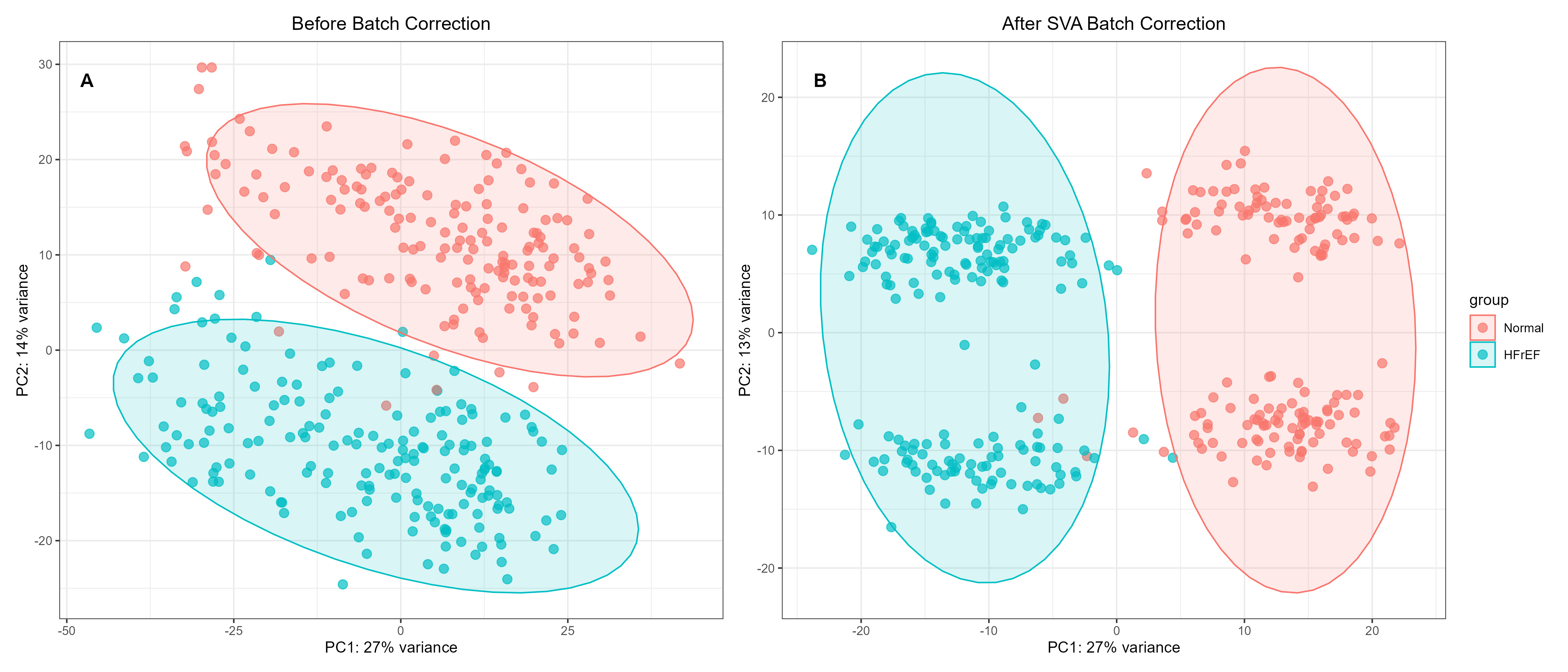
Figure S1. Principal component analysis (PCA) of the GSE141910 transcriptomic dataset before and after batch correction. A: PCA before batch correction, B: PCA after SVA-based batch correction.
Results To evaluate the effectiveness of batch correction on the transcriptomic profiles of the GSE141910 cohort, we performed principal component analysis (PCA) stratified by group (Normal vs. HFrEF). Two‑dimensional PCA plots illustrate sample distribution before (Figure S1A) and after (Figure S1B) Surrogate Variable Analysis (SVA)‑based batch correction, with ellipses representing the 95% confidence intervals for each group. Before correction (Figure S1A), the data already showed partial separation between the Normal and HFrEF groups. However, considerable within‑group dispersion and minor overlap between the 95% confidence ellipses indicated that latent technical variation still contributed to sample scattering and weakened the biological separation. Following SVA‑based batch correction (Figure S1B), the within‑group dispersion was markedly reduced, and the two groups became clearly separated with fully non‑overlapping 95% confidence ellipses. This improved separation demonstrates that the batch correction effectively removed unwanted variation, enhancing the biological signal‑to‑noise ratio and revealing the true transcriptomic difference between the HFrEF and Normal phenotypes. The corrected dataset therefore provides a robust foundation for subsequent differential expression and downstream analyses.
| Home | About | Methods | Previous Module | Next Module |